Sparks Fly
Igniting Fast Data Processing with Advanced File Formats and Serialization

File Formats
In the realm of data storage and processing, file formats play a pivotal role in defining how information is organized, stored, and accessed.
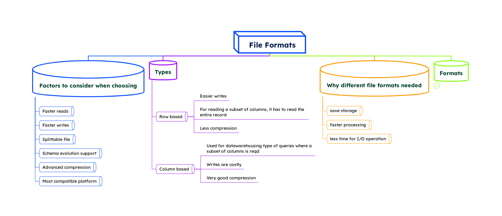
These formats, ranging from simple text files to complex structured formats, serve as the blueprint for data encapsulation, enabling efficient data retrieval, analysis, and interchange. Whether it's the widely used CSV and JSON for straightforward data transactions, or more specialized formats like Avro, ORC, and Parquet designed for high-performance computing environments, each file format brings unique advantages tailored to specific data storage needs and processing workflows.
Comprehensive Snapshot of File Formats
Here's a table summarizing the characteristics, advantages, limitations, and use cases of the mentioned file formats:
| Format | Characteristics | Advantages | Limitations | Use Cases |
| Comma-Separated Values (CSV) | Simple, all data as strings, line-based. | Simplicity, human readability. | Space inefficient, slow I/O for large datasets. | Small datasets, simplicity required. |
| XML/JSON | Hierarchical, complex structures, human-readable. | Suitable for complex data, human-readable. | Non-splittable, can be verbose. | Web services, APIs, configurations. |
| Avro | Row-based, schema in header, write optimized. | Best for schema evolution, write efficiency, landing zone suitability (1), predicate pushdown (2). | Slower reads for subset of columns. | Data lakes, ETL operations, microservices architechture, schema evolving environments. |
| Optimized Row Columnar (ORC) | Columnar, efficient reads, optimized for Hive. | Read efficiency, storage efficiency, predicate pushdown. | Inefficient writes, designed for specific use cases (Hive). | Data warehousing, analytics platforms. |
| Parquet | Columnar, efficient with nested data, self-describing, schema evolution. | Read efficiency, handles nested data, schema evolution, predicate pushdown. | Inefficient writes, complex for simple use cases. | Analytics, machine learning, complex data models. |
(1) Landing zone suitability refers to how well a data storage format or system accommodates the initial collection, storage, and basic processing of raw data in a preparatory or intermediate stage before further analytics or transformation.
(2) Predicate pushdown is an optimization technique that filters data as close to the source as possible, reducing the amount of data processed by pushing down the filter conditions to the storage layer. (ORC, Avro, Parquet)
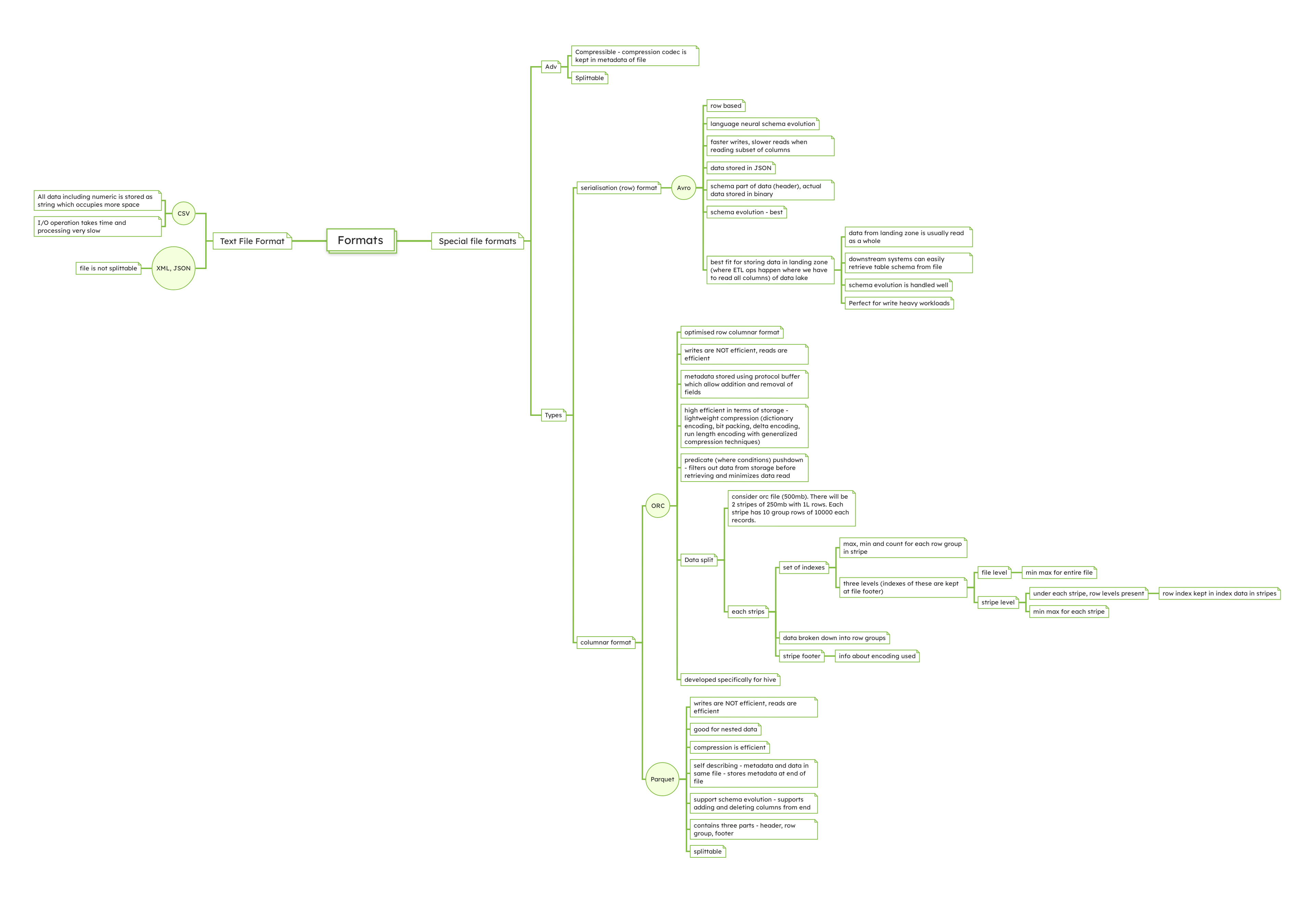
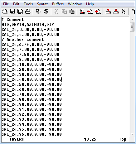
Comma-Separated Values (CSV)
Despite its simplicity, CSV does not enforce any schema, leading to potential issues with data consistency and integrity. It’s extremely flexible but requires careful handling to avoid errors, such as field misalignment or varying data formats.
CSV files can be used as a lowest-common-denominator data exchange format due to their wide support across programming languages, databases, and spreadsheet applications.
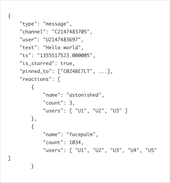
XML/JSON
XML:
XML is highly extensible, allowing developers to create their tags and data structures, but this flexibility can lead to increased file size and complexity.
XML is often used in SOAP-based web services and as a configuration language in many software applications due to its structured and hierarchical nature.
JSON:
JSON's lightweight and text-based structure make it ideal for mobile and web applications where bandwidth may be limited.
JSON has become the preferred choice for RESTful APIs due to its simplicity and ease of use with JavaScript, allowing for seamless data interchange between clients and servers.
Avro: JSON on Steroids
Avro's support for direct mapping to and from JSON makes it easy to understand and use, especially for developers familiar with JSON. This feature enables efficient data serialization without compromising human readability during schema design.
Avro is particularly favored in streaming data architectures, such as Apache Kafka, where schema evolution and efficient data serialization are crucial for handling large volumes of real-time data.
Overview of Avro File Structure
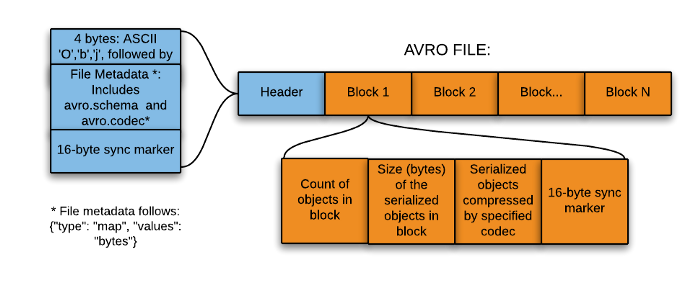
The file structure can be broken down into two main parts: the header and the data blocks.
Header
The header is the first part of the Avro file and contains metadata about the file, including:
Magic Bytes: A sequence of bytes (specifically, "Obj" followed by a null byte) used to identify the file as Avro format.
Metadata: A map (key-value pairs) containing information such as the schema (in JSON format), codec (compression method used, if any), and any other user-defined metadata. The schema in the metadata describes the structure of the data stored in the file, defining fields, data types, and other relevant details.
Sync Marker: A 16-byte, randomly-generated marker used to separate blocks in the file. The same sync marker is used throughout a single Avro file, ensuring that data blocks can be efficiently separated and processed in parallel, if necessary.
Data Blocks
Following the header, the file contains one or more data blocks, each holding a chunk of the actual data:
Block Size and Count: Each block starts with two integers indicating the number of serialized records in the block and the size of the serialized data (in bytes), respectively.
Serialized Data: The actual data, serialized according to the Avro schema defined in the header. The serialization is binary, making it compact and efficient for storage and transmission.
Sync Marker: Each block ends with the same sync marker found in the header, serving as a delimiter to mark the end of a block and facilitate efficient data processing and integrity checks.
Schema Evolution
Schema evolution in Avro allows for backward and forward compatibility, making it possible to modify schemas over time without disrupting existing applications. This feature is critical for long-lived data storage systems and for applications that evolve independently of the data they process.
Backward Compatibility: Older data can be read with a newer schema, enabling applications to evolve without requiring simultaneous updates to all data.
Forward Compatibility: Newer data can be read with an older schema, allowing legacy systems to access updated data formats.
Optimized Row Columnar (ORC)
ORC files include lightweight indexes that store statistics (such as min, max, sum, and count) about the data in each column, allowing for more efficient data retrieval operations. This indexing significantly enhances performance for data warehousing queries.
The format is designed to optimize the performance of Hive queries. By storing data in a columnar format, ORC minimizes the amount of data read from disk, improving query performance, especially for analytical queries that aggregate large volumes of data.
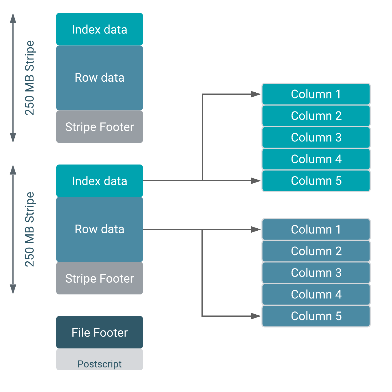
File Structure
An ORC file consists of multiple components, each serving a specific function to enhance storage and query capabilities:
File Header: This section marks the ORC file's beginning, detailing the file format version and other overarching properties.
Stripes: The core data storage units within an ORC file are its stripes, substantial blocks of data usually set between 64MB and 256MB. Stripes contain a subset of the data, compressed and encoded independently, which supports both parallel processing and efficient data access. For example, in a 500MB ORC file, you might find two stripes, each carrying 250MB and consisting of 1 lakh (100,000) rows.
Stripe Header: Holds metadata about the stripe, including the row count, stripe size, and specifics on the stripe's indexes and data streams.
Row Groups: Data within each stripe is organized into row groups, with each grouping a set of rows to be processed collectively. Suppose each stripe is divided into 10 row groups, with each group containing 10,000 records. This structuring facilitates efficient processing by batching the columnar data of several rows.
Column Storage: Within the row groups, data is stored column-wise. Different data types may leverage distinct compression and encoding strategies, optimizing storage and read operations.
Indexes: Integral to ORC's efficiency are the lightweight indexes within each stripe, detailing the contained data. These indexes, including metrics like minimum and maximum values and row counts, enable precise data filtering without necessitating a full data read.
Stripe Footer: Contains detailed metadata about the stripe, such as encoding types per column and stream directories.
File Footer: Summarizes the file by listing stripes and indexes for all levels, detailing the data schema, and aggregating statistics like column row counts and min/max values.
Postscript: Holds file metadata, including encoding and compression details, file footer length, and serialization library versions.
Indexes and Storage Optimization
Each stripe possesses a set of indexes that hold vital data statistics:
File Level: Offers global statistics for the entire file.
Stripe Level: Provides specific statistics for each stripe, facilitating efficient data querying by enabling the system to skip irrelevant stripes.
Row Group Index: Within each stripe, enabling finer control over data access by detailing row group contents.
Parquet
Parquet supports efficient compression and encoding schemes such as dictionary encoding, which can significantly reduce the size of the data stored. This feature makes it an excellent choice for cost-effective storage in cloud environments.
Parquet’s columnar storage model is not just beneficial for analytical querying; it also supports complex nested data structures, making it suitable for semi-structured data like JSON. This adaptability makes it a popular choice for big data ecosystems and data lake architectures, where data comes in various shapes and sizes.
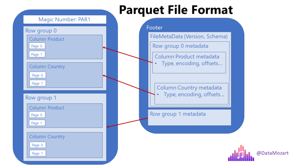
Columnar Storage
Unlike traditional row-based storage, where data is stored as a sequence of rows, Parquet stores data in a columnar format. This means each column is stored separately, enabling more efficient data retrieval and compression, especially for analytical workloads where only a subset of columns may be needed for a query.
Row Groups
Similar to row groups in stripes in the ORC format, a row group in Parquet is a vertical partitioning of data into columns within a certain chunk of rows. This organization allows for both columnar storage benefits and efficient data scanning across rows.
Let's make this a little clearer- The data is organized into columns that are further divided into row groups. Each row group contains a segment of the dataset's rows, but stores this data in a column-oriented manner.
Example Scenario
Let's take an example where data about products and countries is stored in Parquet format. In a traditional row store, a query filtering for specific product types and countries would need to scan every row. However, with Parquet's structure, the engine can directly access the columns for products and countries, and within those, only the row groups relevant to the query criteria, significantly reducing the amount of data processed. (Reference for a better understanding- Data Mozart's article on Parquet)
Efficiency in Analytical Queries
Projection and Predicate Pushdown
Parquet's file structure is particularly advantageous for analytical queries that involve projection (selecting specific columns) and predicates (applying filters on rows). The columnar storage allows for projection by accessing only the needed columns, while the row groups facilitate predicate pushdown by enabling selective scanning of rows based on the filters applied.
Metadata
Metadata in Parquet files includes details about the data's structure, such as schema information, and statistics about the data stored within the file.
Facilitating Data Skips
With metadata, query engines can perform optimizations such as predicate pushdown. By providing detailed information about the data's organization and content, the metadata allows query engines to quickly determine which parts of the data need to be read and which can be skipped.
Reducing I/O Operations
By minimizing the need to read irrelevant data from disk, metadata significantly reduces I/O operations, a common bottleneck in data processing. This efficiency is crucial for handling large datasets where reading the entire dataset from disk would be prohibitively time-consuming and resource-intensive.
Metadata Structure
Every Parquet file contains a footer section, which holds the metadata. This includes format version, schema information and column metadata like statistics for individual columns within each row group.
Encoding
Run Length Encoding (RLE)
Run-Length Encoding is a straightforward yet powerful compression technique. Its primary objective is to reduce the size of data that has numerous repeatitive occurrences of the same value (runs). Instead of storing each value individually, RLE compresses a run of data into two elements: the value itself and the count of how many times the value repeats consecutively.
Identification of Runs: RLE scans the data to identify runs, which are sequences where the same value occurs consecutively.
Compression: Each run is then compressed into a pair: the value and its count. For example, the sequence
AAAABBBCCis compressed toA4B3C2.Efficiency: The efficiency of RLE is highly dependent on the data's nature. It performs exceptionally well on data with many long runs but might not be effective for data with high variability.
Run Length Encoding with Bit Packing
Combining RLE with bit-packing enhances its compression capability, especially for numerical data with a limited range of values. Bit-packing is a technique that minimizes the number of bits needed to represent a value, packing multiple numbers into a single byte or word in memory.
Let me expand on bit-packing a little more to make it easier.
A byte consists of 8 bits, and traditionally, a whole byte might be used to store a single piece of information. But if your information can be represented with fewer bits, you can store multiple pieces of information in the same byte.
For example, for integers ranging from 0 to 15, you only need 4 bits to represent all possible values. Why? Because 4 bits can create 16 different combinations (2^4). Here’s how the bit representation looks for these numbers:
The number 0 is
0000in binary.The number 1 is
0001....
The number 15 is
1111.
Each of these can fit in just half a byte (or 4 bits).
Now, instead of using a whole byte (8 bits) for each number, you decide to pack two numbers into one byte.
Let's consider you have the numbers 3 (0011) and 14 (1110) to store:
Convert each number to its 4-bit binary representation:
0011for 3 and1110for 14.Pack these two sets of 4 bits into one byte:
00111110.
If you are considering actual values from bit packing beyond the scope of the example above (repeats greater than 15), then you either split the runs or use a flag to identify only those run lengths and then display the exact number of repeats after that.
Now, when RLE is combined with bit-packing, it efficiently compresses runs of integers by first using RLE to encode the run lengths and then applying bit-packing to compress the actual values. This dual approach is particularly effective for numerical data with small ranges or repetitive sequences.
RLE on Runs: Identifies and encodes the length of runs.
Bit-Packing on Values: Applies bit-packing to the values themselves, further reducing the storage space required.
Use Case Example: A sequence of integers with many repeats and a small range, such as
[0, 0, 0, 1, 1, 2, 2, 2, 2], would first have RLE applied to compress the repeats, then bit-packing could compress the actual numbers since they require very few bits to represent.
Dictionary Encoding
Dictionary encoding is a compression technique where a unique dictionary is created for a dataset, mapping each distinct value to a unique integer identifier. This approach is highly effective in datasets with many unique records, but they repeat a few specific values often.
Dictionary Creation: Scan the dataset to identify all unique values. Each unique value is assigned a unique integer identifier. This mapping of values to identifiers forms the dictionary.
Data Transformation: Replace each value in the dataset with its corresponding identifier from the dictionary. This results in a transformed dataset where repetitive values are replaced with their integer identifiers, often much smaller in size than the original values.
Storage: The dictionary and the transformed dataset are stored together. To reconstruct the original data, a lookup in the dictionary is performed using the integer identifiers.
Example: Consider a column with the values ["Red", "Blue", "Red", "Green", "Blue"]. A dictionary might map these colors to integers as follows: {"Red": 1, "Blue": 2, "Green": 3}. The encoded column becomes [1, 2, 1, 3, 2].
Dictionary Encoding with Bit Packing
If the range of unique integers is small, you can further compress this data with bit-packing.
Apply Dictionary Encoding: First, create a dictionary for the column's unique values, assigning each an integer identifier. Replace each original value in the column with its corresponding identifier.
Assess the Dictionary Size: Determine the maximum identifier value used in your dictionary. This tells you the range of values you need to encode.
Determine Bit Requirements: Calculate the minimum number of bits required to represent the highest identifier. For example, if your highest identifier is 15, you need 4 bits.
Bit-Pack the Identifiers: Instead of storing these identifiers using standard byte or integer formats, you pack them into the minimum bit spaces determined. This might mean putting two 4-bit identifiers into a single 8-bit byte, effectively doubling the storage efficiency for these values. (Similar to what we went over in the 3 (
0011) and 14 (1110) example above)
Data Serialization
Having explored file formats, our focus shifts to the critical aspect of how we mobilize this data. This is where serialization comes in- it acts as the conduit or channel, transforming data structures and objects into a streamlined sequence of bytes that can be easily stored, transmitted, and subsequently reassembled.
Spark uses serialization to:
Transfer data across the network between different nodes in a cluster.
Save data to disk when necessary, such as persisting RDDs (which will be discussed in the future articles) or when spilling data from memory to disk during shuffles.
Serialization Libraries
Spark supports two main serialization libraries:
Java Serialization Library
Default Method: The default serialization method used by Spark is the native Java serialization facilitated by implementing the
java.io.Serializableinterface.Ease of Use: This method is straightforward to use since it requires minimal code changes, but it can be relatively slow and produce larger serialized objects, which may not be ideal for network transmission or disk storage.
Kryo Serialization Library
Performance-Optimized: Kryo is a faster and more compact serialization framework compared to Java serialization. It can significantly reduce the amount of data that needs to be transferred over the network or stored.
Configuration Required: To use Kryo serialization, it must be explicitly enabled and configured in Spark. This involves registering the classes you'll serialize with Kryo, which can be a bit more work but is often worth the effort for the performance gains.
Implementation and Use Cases
Configuring Spark for Serialization: In Spark, you can configure the serialization library at the start of your application through the Spark configuration settings, using
spark.serializerproperty. For Kryo, you would set this toorg.apache.spark.serializer.KryoSerializer.Serialization for Performance: Choosing the right serialization library and tuning your configuration can have a significant impact on the performance of your Spark applications, especially in data-intensive operations. Efficient serialization reduces the overhead of shuffling data between Spark workers and nodes, and when persisting data.
Best Practices
Use Kryo for Large Datasets: For applications that process large volumes of data or require extensive network communication, using Kryo serialization is recommended.
Register Classes with Kryo: When using Kryo, explicitly registering your classes can improve performance further, as it allows Kryo to optimize serialization and deserialization operations.
Tune Spark’s Memory Management: Properly configuring memory management in Spark, alongside efficient serialization, can reduce the occurrence of spills to disk and out-of-memory errors, leading to smoother and faster execution of Spark jobs. We'll discuss more on memory management in the upcoming articles.
Whether encoding data in JSON for web transport, using Avro for its compact binary efficiency, or adopting Parquet's columnar approach for analytic processing, the method of serialization chosen is pivotal. It not only dictates the ease and efficiency of data movement but also shapes how data is preserved, accessed, and utilized across various platforms and applications.
Deserialization: Putting the puzzle back together
After detailing the serialization process, it's essential to understand its counterpart: deserialization. Deserialization reverses serialization's actions, converting the sequence of bytes back into the original data structure or object. This process is crucial for retrieving serialized data from storage or after transmission, allowing it to be utilized effectively within applications.
Spark's Approach to Deserialization
In Apache Spark, deserialization plays a vital role in:
Reading Data from Disk: When data persisted in storage (like RDDs or datasets) needs to be accessed for computation, Spark deserializes it into the original format for processing.
Receiving Data Across the Network: Data sent between nodes in a cluster is deserialized upon receipt to be used in computations or stored efficiently.
Deserialization Libraries in Spark
As with serialization, Spark leverages the same libraries for deserialization:
Java Deserialization: By default, Spark uses Java’s built-in deserialization mechanism. This method is automatically applied to data serialized with Java serialization, ensuring compatibility and ease of use but may carry performance and size overheads.
Kryo Deserialization: For data serialized with Kryo, Spark employs Kryo’s deserialization methods, which are designed for high performance and efficiency. Similar to serialization, proper configuration and class registration are essential for leveraging Kryo's full potential in deserialization processes.
Implementing Deserialization in Spark Applications
Configuration for Deserialization: Similar to serialization, deserialization settings in Spark are configured at the application's outset via Spark configuration. Ensuring that the deserialization library matches the serialization method used is crucial for correct data retrieval.
Deserialization for Data Recovery and Processing: Effective deserialization is key for the rapid recovery of persisted data and the efficient execution of distributed computations, impacting overall application performance.
Best Practices for Deserialization
Match Serialization and Deserialization Libraries: Ensure consistency between serialization and deserialization methods to avoid errors and data loss.
Optimize Data Structures for Serialization/Deserialization: Design data structures with serialization efficiency in mind, particularly for applications with heavy data exchange or persistence requirements.
Monitor Performance Impacts: Regularly assess the impact of serialization and deserialization on application performance, adjusting configurations as necessary to optimize speed and resource usage.
Serialization between Memory and Disk
Serialization: Before writing data to disk, Spark serializes the data into a binary format. This is done to minimize the memory footprint and optimize disk I/O.
Spilling: When the memory usage exceeds the available memory threshold, Spark spills data to disk to free up memory. This spilled data, in its serialized form, is written to disk partitions, typically in temporary spill files.
Deserialization: When the spilled data needs to be read back into memory for further processing, Spark deserializes the data from its binary format back into objects.
The interplay between serialization and deserialization is a foundational aspect of data processing in distributed systems like Apache Spark- while serialization ensures that data is efficiently prepared for transfer or storage, deserialization makes that data usable again, completing the cycle of data mobility. As we continue exploring Spark's advanced capabilities and optimizations in future articles, the importance of efficient serialization and deserialization practices in enhancing performance and enabling complex computations over distributed data will become increasingly apparent.