


Table of contents
In the vast world of big data processing, Apache Hive has emerged as a powerful tool for querying and analyzing large datasets stored in distributed storage systems like Hadoop. However, as the volume and complexity of data continue to grow, optimizing Hive's performance becomes crucial. In this article, we will delve into the realm of hive optimization, exploring various strategies and techniques to boost query performance and maximize the efficiency of your data processing pipeline.
Structure Level Optimization
Optimizing Hive for maximum performance requires not only writing better queries but paying attention to schema and structure. By carefully designing data models, balancing normalization and denormalization, and considering factors like bucketing, partitioning, indexing, and compression, you can significantly improve the performance of your Hive environment. Let's dive into bucketing and partitioning.
Partitioning
Partitioning involves dividing a table into smaller, more manageable parts based on a particular column or set of columns. This can help with data organization, querying, and filtering. I will go over the two types of partitioning - Static and Dynamic Partitioning. I will also dive into a common issue with partitioning - Over Partitioning.
Static Partitioning
In static partitioning, the partition values are explicitly specified manually during the data insertion process. Static partitions require prior knowledge of the partition values, and separate INSERT statements are needed for each partition. It provides better control and predictability over partitioning as the partitions are pre-defined and known in advance. Static partitions are typically suitable for scenarios where the partitioning criteria are well-defined and stable, such as partitioning data by year or region.
Dynamic Partitioning
Dynamic partitioning, also known as automatic partitioning, allows Hive to automatically determine the partitions based on the values present in the data being inserted. With dynamic partitions, a single INSERT statement can insert data into multiple partitions without explicitly specifying partition values. Dynamic partitions are flexible and can adapt to changes in data without requiring manual intervention. This type of partitioning is useful when the partitioning criteria are not known in advance or when new partitions need to be created frequently, such as partitioning data by date or customer ID.
Dealing With Over Partitioning
When working with Hive and HDFS, it's important to consider the drawbacks of having too many partitions. The creation of numerous Hadoop files and directories for each partition can quickly overwhelm the NameNode's capacity to manage the filesystem metadata. As the number of partitions grows, the strain on memory and the potential for exhausting metadata capacity increases.
Additionally, MapReduce processing introduces overhead in the form of JVM start-up and tear-down, which can be significant when dealing with small files.
When implementing time-range partitioning in Hive, it is recommended to estimate the data size across different time granularities. Begin with a granularity that ensures controlled partition growth over time, while ensuring that each partition's file size is at least equal to the filesystem block size or its multiples. This approach optimizes query performance for general queries. However, it's crucial to consider when the next level of granularity becomes appropriate, particularly if query WHERE clauses often select ranges of smaller granularities.
Another approach is to employ two levels of partitions based on different dimensions. For example, you can partition by day at the first level and by geographic region (e.g., state) at the second level. This allows for more targeted querying, such as retrieving data for a specific day within a particular state.
However, it is worth noting that processing imbalances may occur when handling larger states that have significantly more data, resulting in longer processing times compared to smaller states with lesser data volumes. This is where bucketing comes into the picture.
Bucketing
Bucketing involves grouping data based on a hash function applied to one or more columns. This can improve query performance by reducing the amount of data that needs to be scanned.
Use Case
Partitioning is a useful technique when the cardinality or number of unique values in a column is low. For example, if you have a table of sales data with a "year" column, partitioning the data based on this column can make it easier to filter and analyze sales for specific years.
Bucketing, on the other hand, is ideal when the cardinality of a column is high.
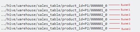
See the image below on how Hive stores partitions and buckets. There are two partitions based on product ID (P1 and P2) and 3 buckets (bucket 0, bucket 1 and bucket 2).
- Use the function -
SHOW PARTITIONS sales_table
to see all the partitions in your table.
- Use the following query to see the bucket
SELECT * FROM sales_table TABLESAMPLE (bucket 1 out of 3);
Change the bucket number to 1, 2 and 3 to see the data in each bucket.
Query Level Optimization
Join optimization techniques in Hive aim to improve the performance and efficiency of join operations, which are essential for querying and analyzing large datasets.
Join optimization techniques in Hive involve the use of hashtables and leveraging distributed processing to improve performance. The process generally follows these steps:
A hashtable is created from the smaller table involved in the join operation.
The hashtable is moved to HDFS for storage and accessibility.
From HDFS, the hashtable is broadcasted to all nodes in the cluster, ensuring it is available locally.
The hashtable is then stored in the distributed cache, residing on the local disk of each node.
Each node loads the hashtable into memory from its local disk, allowing for efficient in-memory access.
Finally, the MapReduce job is invoked to perform the join operation, utilizing the loaded hashtables to optimize the process.
Here is a summary of common join optimization techniques used in Hive:
Map Side Join Optimization
In certain cases, if one of the tables being joined is small enough to fit in memory, Hive can perform a map-side join. This technique avoids costly shuffling and reduces the need for network transfers by distributing the smaller table to all mapper tasks.
Settings
SET hive.auto.convert.join=true; -- default true after v0.11.0
SET hive.mapjoin.smalltable.filesize=600000000; -- default 25m
SET hive.auto.convert.join.noconditionaltask=true; -- default value above is true so map join hint is not needed
SET hive.auto.convert.join.noconditionaltask.size=10000000; -- default value above controls the size of table to fit in memory
With join auto-convert enabled in Hive, the system will automatically assess if the file size of the smaller table exceeds the specified threshold defined by hive.mapjoin.smalltable.filesize. If the file size is smaller than the threshold, Hive will attempt to convert the common join into a map join. This automatic conversion eliminates the need to explicitly provide map join hints in the query, simplifying the query writing process and reducing manual optimization efforts. By leveraging this feature, users can optimize join operations without the need for manual intervention.
Code
-- Perform a map join on two tables
SELECT  /*+ MAPJOIN(table2) */ *
FROM table1
JOIN table2 ON table1.key = table2.key;
Conditions
- Except for one big table, all other tables in the join operation should be small.
Here is a quick guide for the different joins and which table should be the smaller one.
| Type of join | Small table |
| Inner Join | Left table must be small |
| Left Join | Right table must be small |
| Right Join | Left table must be small |
| Full Outer Join | Cannot be treated as a map side join |
Bucket Map Join Optimization
When both tables are bucketed on the join key, Hive can leverage bucketed map joins. This technique allows data with the same bucket ID to be processed locally, minimizing data movement and reducing the need for a full shuffle.
It's important to note that unlike map side join,
it can be done on two big tables.
Only one bucket is loaded in memory essentially.
Settings
SET hive.auto.convert.join=true;
SET hive.optimize.bucketmapjoin=true; -- default false
Code
-- Perform a bucketed map join on two tables
SELECT /*+ MAPJOIN(table2) */ *
FROM table1
JOIN table2 ON table1.key = table2.key
CLUSTERED BY (key) INTO <num_of_buckets>;
Conditions
Both tables should be bucketed on the join column.
Join tables must have integral multiple of buckets. Eg - If table 1 has 4 buckets, table 2 can have 4,8,12, etc buckets.
Sort Merge Bucket Join Optimization
When both tables are bucketed and sorted on the join key, Hive can use sort merge bucketed joins. This technique avoids unnecessary data shuffling and performs an efficient merge operation on the sorted buckets, enhancing join performance. This join can be done on two big tables.
Settings
SET hive.input.format= org.apache.hadoop.hive.ql.io.BucketizedHiveInputFormat;
SET hive.auto.convert.sortmerge.join=true;
SET hive.optimize.bucketmapjoin=true;
SET hive.optimize.bucketmapjoin.sortedmerge=true;
SET hive.auto.convert.sortmerge.join.noconditionaltask=true;
Code
-- Perform a sort merge bucketed join on two tables
SELECT /*+ SMBJOIN(table2) */ *
FROM table1
JOIN table2 ON table1.key = table2.key
CLUSTERED BY (key) SORTED BY (key) INTO <num_of_buckets>;
Conditions
Both tables should be bucketed on the join column.
The number of buckets in one table must be equal to the number of buckets in the other table.
Both tables should be sorted based on the join column.
Sort Merge Bucket Map Join Optimization
An SMBM (Sort-Merge-Bucket-Merge) join is a specific type of bucket join that exclusively triggers a map-side join. Unlike a traditional map join that requires caching all rows in memory, an SMBM join avoids this overhead.
Settings
SET hive.auto.convert.sortmerge.join=true
SET hive.optimize.bucketmapjoin=true;
SET hive.optimize.bucketmapjoin.sortedmerge=true;
SET hive.auto.convert.sortmerge.join.noconditionaltask=true;
SET hive.auto.convert.sortmerge.join.bigtable.selection.policy= org.apache.hadoop.hive.ql.optimizer.TableSizeBasedBigTableSelectorForAutoSM J;
Conditions
Both tables should be bucketed on the join column.
The number of buckets in one table must be equal to the number of buckets in the other table.
Both tables should be sorted based on the join column.
Skew Join Optimization
When dealing with data that exhibits a significant imbalance in distribution, data skew can occur, leading to a situation where a few compute nodes bear the brunt of the computation workload.
Settings
SET hive.optimize.skewjoin=true; --If there is data skew in join, set it to true. Default is false.
SET hive.skewjoin.key=100000; --This is the default value. If the number of key is bigger than --this, the new keys will send to the other unused reducers.
SET hive.groupby.skewindata=true;
Data skew can also occur when performing GROUP BY operations, leading to uneven distribution and performance bottlenecks. To address this, Hive offers the setting above, enabling skew data optimization specifically for GROUP BY results. Once enabled, Hive initiates an additional MapReduce job that strategically redistributes the map output across reducers in a random manner, effectively mitigating data skew and improving overall query performance. By configuring this setting, Hive ensures a more balanced workload distribution and optimized processing for GROUP BY operations affected by skewed data.
Code
-- Perform a join with skew join optimization
SELECT /*+ SKEWJOIN(table1) */ *
FROM table1
JOIN table2 ON table1.key = table2.key;